1. Statistics Fundamentals

1.1. Descriptive Statistics

• P-value: the probability that we'd observe an extreme or more extreme statistic than we did given the null hypothesis was true.

• Expected value: weighted average of each case. Expected value use probability to tell us what outcomes to expect in the long run.

• Variance: the sum of the squared distance from the data to the mean

• Median

• Mode

• Percentile/Quartiles/Deciles

• Outlier: 

  • 1.5 IQR rule for outliers - a data point is an outlier if it's more than 1.5 IQR above the 3rd quartile or below the 1st quartile

1.2. Law of Large Numbers (LLN)

In probability theory, the LLN is a theorem that describes the results of performing the same experiment a large number of times. According to the law, the average of the results obtained from a large number of trials should be close to the expected value, and will tend to become closer as more trials are performed.

1.3. Central Limit Theorem (CLT)

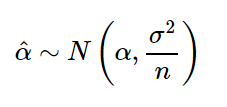
As the sample size becomes larger, the sample mean distribution (sampling distribution) will be closed to normal distribution, no matter what the shape of the population distribution. 

• Sample Sum distribution ~ N (μ', σ'):
  • μ' = n * μ
  • σ' = σ * n**(1/2)
• Sample Mean distribution ~ N (μ', σ'):
  • μ' = μ
  • σ' = σ / n**(1/2)

1.4. Matrix Determinant 

1.4.1. 3x3 matrix

\[ \det \begin{pmatrix}a&b&c\\ d&e&f\\ g&h&i\end{pmatrix}=a\cdot \det \begin{pmatrix}e&f\\ h&i\end{pmatrix}-b\cdot \det \begin{pmatrix}d&f\\ g&i\end{pmatrix}+c\cdot \det \begin{pmatrix}d&e\\ g&h\end{pmatrix} \]

---

2. Hypothesis Testing

2.1. Terms

• P-value: Given null hypothesis is true, the probability of observed outcomes
• Confidence Interval: The range within which the mean is expected to fall in multiple trails of the experiment.
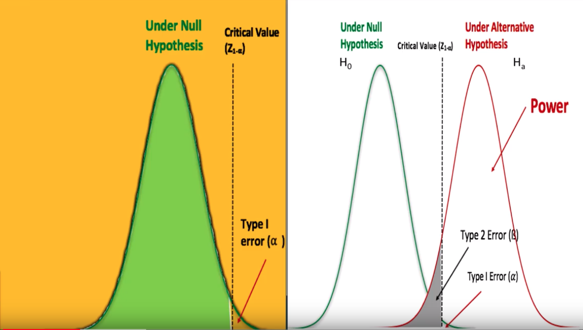
• Type-I error: (α) Falsely reject a true null hypothesis – False positive

• Type-II error: (β) Fail to reject a a false null hypothesis – False negative

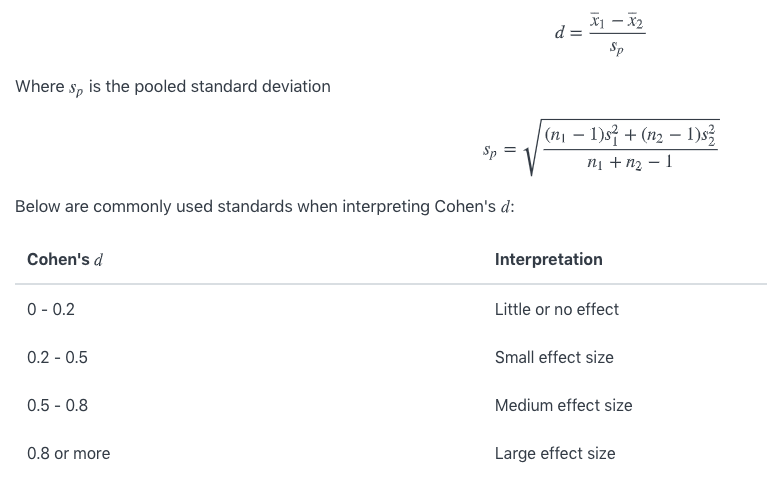
  	True Null Hypothesis	False Null Hypothesis
  Reject Null Hypothesis	Type-I error (α)	correct (power)
  Accept Null Hypothesis	correct	Type-II error(β)

• Practical Significance: The magnitude of the difference. Can be examined by computing Cohen's d, which is the difference between the two observed sample means in standard deviation units: 

2.2. Power in significance test:

Power = 1-β = Pr(Rejecting null hypo | Null hypo is false) = 1 - Pr(Accept null hypo | Null hypo is false) = Pr(Not making Type-II error) 

Usually choose 0.8 or higher power.

Four primary factors affect power:

1. • Significance level (α)
   • Sample size (n)
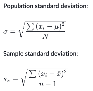
   • Variability, or variance, in the measured response variable (σ or s)
   • Magnitude of the effect of the variable (effect size ε)

2.3. Sample Size

https://online.stat.psu.edu/stat414/node/306/

Estimate sample size given desired alpha and beta.

2.3.1. Estimating a mean

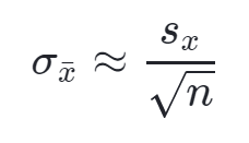
• The sample size necessary for estimating a population mean μ with (1−α)100% confidence and error no larger than ε is:

    where we can use z_α/2 to replace t_{α/2, n-1 .}   

• How to estimate s? – Empirical Rule  

    

2.3.2. Estimating a proportion for a large population

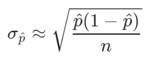
• An approximate (1−α)100% confidence interval for a proportion p of a large population is:

\[ \hat{p}\pm z_{\alpha/2}\sqrt{\dfrac{\hat{p}(1-\hat{p})}{n}} \]

• The sample size necessary for estimating a population proportion p of a large population with (1−α)100% confidence and error no larger than ε is:

\[ n=\dfrac{z^2_{\alpha/2}\hat{p}(1-\hat{p})}{\epsilon^2} \]

• How to estimate 

  \[ \hat{p}(1-\hat{p}) \]

  Set p(1-p) = 1/4, its maximum when p = 1/2

2.3.3. Estimating a proportion for a small population (N is small)

• An approximate (1−α)100% confidence interval for a proportion p of a small population is:

  \[ \hat{p}\pm z_{\alpha/2}\sqrt{\dfrac{\hat{p}(1-\hat{p})}{n} \cdot \dfrac{N-n}{N-1}} \]

  Noting that if the sample n is much smaller than the population size N, that is, if n << N, then (N-n)/(N-1) ≈ 1, and the confidence interval for p of a small population becomes quite similar to the confidence interval for p of a large population.

  
  

• The sample size necessary for estimating a population proportion p of a small finite population N with (1−α)100% confidence and error no larger than ε is:

  \[ n=\dfrac{z^2_{\alpha/2}\hat{p}(1-\hat{p})/\epsilon^2}{\dfrac{N-1}{N}+\dfrac{z^2_{\alpha/2}\hat{p}(1-\hat{p})}{N\epsilon^2}} \]

  or

  \[ n=\dfrac{m}{1+\dfrac{m-1}{N}} \]

  where

  \[ m=\dfrac{z^2_{\alpha/2}\hat{p}(1-\hat{p})}{\epsilon^2} \]

  
  

2.4. Steps

1. Write hypothesis
2. Check conditions (Random, Normal, Independence)
3. Calculate t or z statistics
4. Get p-value (one-tailed or two-tailed)
5. Compare p-value to α (significance level)
   1. Type-I or Type-II error
   2. Power
6. Make a conclusion

2.5. Types

2.5.1. Test on a population proportion

• Conditions for a z-test:
  • Random: the data needs to come from a random sample or randomized experiment.
  • Normal: the sampling distribution of p (the sample proportion) needs to be approximately normal – needs at least 10 expected successes and 10 expected failures:
    • np >= 10
    • n(1-p) >= 10
  • Independence: individual observation needs to be independent. If sampling without replacement, the sample size shouldn't be more than 10% of the population:
    
    • use replacement
    • OR n <= 10% population
• Calculate a z statistic: Delta / Std Error

2.5.2. Test on a population mean

• Conditions for a z-test:
  • Random: a random sampling or randomized experiment should be used to obtain the data
  • Normal: the sampling distribution of x (the sample mean) needs to be approximately normal. It is true if the parent population is normal or if the sample size is reasonably large (n >= 30):
    • parent population is normal
    • OR n >= 30
    • OR if unknown parent population distribution and n < 30 – the big idea is that we need to graph the sample data when n < 30 and make a decision about the normal condition based on the appearance of the sample data (symmetric without outlier)
  • Independence: Individual observation needs to be independent. If sampling without replacement, the sample size shouldn't be more than 10% of the population:
    • use replacement
    • OR n <= 10% of population
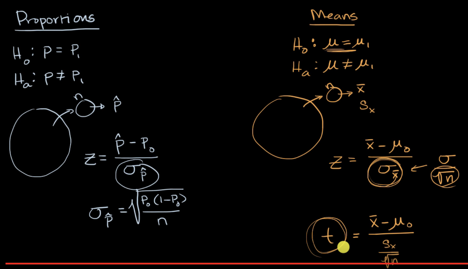
• Calculate a z or t statistics: Delta / Std Error  
• When to use z or t statistic:
  • if known population variance, use population standard deviation: z statistic
  • if DON'T known population variance, use sample standard deviation: t statistic
    
        

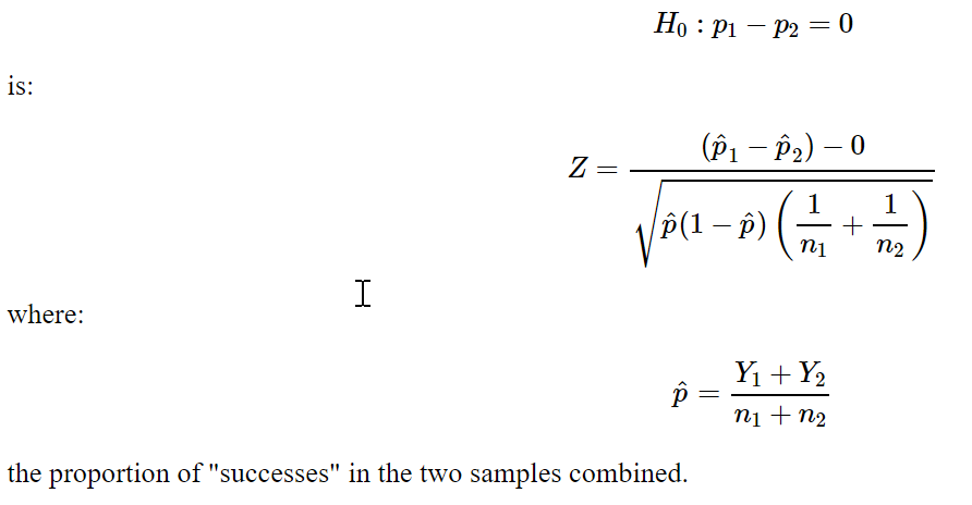
2.5.3. Test on two sample proportions

• Calculate z statistic: Delta / Std Error

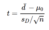
2.5.4. Test on paired means

• In this situation, our measurements differences are di, df = n-1
• calculate t statistic: Delta / Std Error  

2.5.5. Test on two independent sample means

• When population variances are equal:
  • df = n+m-1

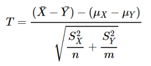
  • calculate t statistic: Delta / Std Error  ,  

    
    

• When population variances are not equal:

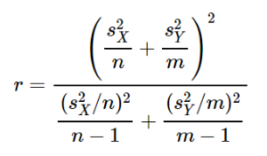
  • adjusted df (integer portion of r): 

  • calculate t statistic: Delta / Std Error 

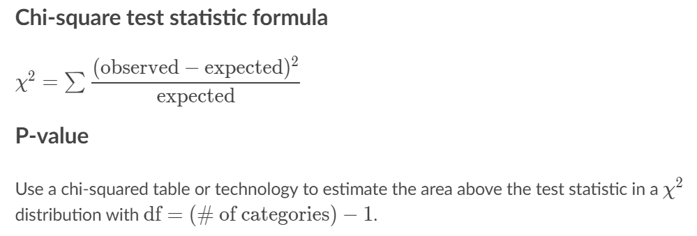
2.5.6. Test on the distribution of categorical data: Chi-squared test χ^₂ 

• Data come from one sample → test of independence
• Data come from separate samples → test of homogeneity
• Conditions:
  • Random
  • Normal: Large number (>= 5 per cell)
  • Independence: (sample <= 10% of population)
• Goodness-of-fit test:
  • df = n-1
• Relationship test:
  • df = (# of rows - 1)*(# of columns - 1)
• Two variable association test:
  • df = (# of rows - 1)*(# of columns - 1)
    
    

2.5.7. Test on one variance: Chi-squared test χ^₂ 

If you have a random sample of size n from a normal population with (unknown) mean μ and variance σ², then:

\[ \chi^2=\dfrac{(n-1)S^2}{\sigma^2} \]

follows a chi-square distribution with n−1 degrees of freedom.

2.5.8. Test on two variance: F-test

Can be used to test the validation of the assumption of equal variance that needs when performing two-sample t-test.

follows an F distribution with  n−1 numerator degrees of freedom and m−1 denominator degrees of freedom.

If we're interested in testing the null hypothesis:

\[ \chi^2=\dfrac{(n-1)S^2}{\sigma^2} \]

against any of the alternative hypotheses:

\[ H_A:\sigma^2_X \neq \sigma^2_Y,\quad H_A:\sigma^2_X >\sigma^2_Y,\text{ or }H_A:\sigma^2_X <\sigma^2_Y \]

we can use the test statistic:

\[ F=\dfrac{S^2_X}{S^2_Y} \]

and follow the standard hypothesis testing procedures. When doing so, we might also want to recall this important fact about the F-distribution:

\[ F_{1-(\alpha/2)}(n-1,m-1)=\dfrac{1}{F_{\alpha/2}(m-1,n-1)} \]

so that when we use the critical value approach for a two-sided alternative:

\[ H_A:\sigma^2_X \neq \sigma^2_Y \]

we reject if the test statistic F is too large:

\[ F \geq F_{\alpha/2}(n-1,m-1) \]

or if the test statistic F is too small:

\[ F \leq F_{1-(\alpha/2)}(n-1,m-1)=\dfrac{1}{F_{\alpha/2}(m-1,n-1)} \]

3. ANOVA

3.1. Assumptions

• Independence
• Normality
• Equal group variances

3.2. ANOVA Table

• Analysis of variance, is a collection of methods for comparing multiple means across different groups
• y groups, x samples in each group:
  • SST – Total Sum of Squares (df = x * y - 1)
  • SSW – Total Sum of Squares Within (df = y * (x-1))
  • SSB - Total Sum of Squares Between (df = y - 1)
  • SST = SSW + SSB

\[ SS(E)=\sum\limits_{i=1}^{m}\sum\limits_{j=1}^{n_i} (X_{ij}-\bar{X}_{i.})^2 \] \[ SS(T)=\sum\limits_{i=1}^{m}\sum\limits_{j=1}^{n_i}(\bar{X}_{i.}-\bar{X}_{..})^2 \] \[ SS(TO)=\sum\limits_{i=1}^{m}\sum\limits_{j=1}^{n_i} (X_{ij}-\bar{X}_{..})^2 \]

• If X_ij ~ N(μ, σ²), then:

  \[ F=\dfrac{SST/(m-1)}{SSE/(n-m)}=\dfrac{MST}{MSE} \sim F(m-1,n-m) \]

4. Linear Models

4.1. Assumptions (LINE):

• The mean of the responses, E(Y_i), is a Linear function of the x_i.
• The errors, ε_i, and hence the responses Y_i, are Independent.
• The errors, ε_i, and hence the responses Y_i, are Normally distributed.
• The errors, ε_i, and hence the responses Y_i, have Equal variances (σ²) for all x values.

4.2. Least-Squares Linear Regression

• Y = βx + α
  • β = r*(s_y/s_x) = s_x*s_y/s_xx

4.3. Ordinary Least Squares (OLS) vs Gradient Descent (GD)

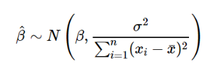
• The OLS estimate the slope 𝛽 and intercept 𝛼 of the straight line by minimizing the sum of squared residuals (SSE).
  
  
  
  
  

• Gradient descent approach aims to minimize a cost function by iterations. The cost function for the simple linear regression is equivalent to the average of squared residuals.
   where m is the batch size.

   where α is a learning rate / how big a step take to downhill.

4.3.1. Types of gradient descent

4.3.1.1. Batch Gradient Descent

• In the batch gradient descent, to calculate the gradient of the cost function, we need to sum all training examples for each steps
• If we have 3 millions samples (m training examples) then the gradient descent algorithm should sum 3 millions samples for every epoch. To move a single step, we have to calculate each with 3 million times!
• Batch Gradient Descent is not good fit for large datasets

4.3.1.2. Stochastic Gradient Descent (SGD)

• In stochastic Gradient Descent, we use one example or one training sample at each iteration instead of using whole dataset to sum all for every steps
• SGD is widely used for larger dataset trainings and computationally faster and can be trained in parallel
• Need to randomly shuffle the training examples before calculating it

4.3.1.3. Mini-Batch Gradient Descent

• It is similar like SGD, it uses n samples instead of 1 at each iteration.

4.4. L1 & L2 Regularization 

• L1 - LASSO
  • Subjective function: min∑(𝑦 −𝑥𝛽)² +𝜆∑|𝛽|
• L2 - Ridge
  • Subjective function: min∑(𝑦 −𝑥𝛽)² +𝜆∑𝛽² 

5. Logistic Regression

5.1. Assumptions

1. APPROPRIATE OUTCOME STRUCTURE: Binary logistic regression requires the dependent variable to be binary and ordinal logistic regression requires the dependent variable to be ordinal.
2. OBSERVATION INDEPENDENCE: Logistic regression requires the observations to be independent of each other.  In other words, the observations should not come from repeated measurements or matched data.
3. THE ABSENCE OF MULTICOLLINEARITY: Logistic regression requires there to be little or no multicollinearity among the independent variables. This means that the independent variables should not be too highly correlated with each other.
4. LINEARITY OF INDEPENDENT VARIABLES AND LOG ODDS: Logistic regression assumes linearity of independent variables and log odds. Although this analysis does not require the dependent and independent variables to be related linearly, it requires that the independent variables are linearly related to the log odds.
5. A LARGE SAMPLE SIZE: Logistic regression typically requires a large sample size. A general guideline is that you need at minimum of 10 cases with the least frequent outcome for each independent variable in your model. For example, if you have 5 independent variables and the expected probability of your least frequent outcome is .10, then you would need a minimum sample size of 500= (10*5 / .10).

5.2. Definitions

5.2.1. Odds

Showing that odds are ratios.

     odds = p/(1 - p)

5.2.2. Log Odds

Natural log of the odds, also known as a logit.

     log odds = logit = log(p/(1 - p))

5.2.3. Odds Ratio

Showing that odds ratios are actually ratios of ratios.

                  odds1     p1/(1 - p1)
     odds_ratio = ----- = -------------
                  odds2     p2/(1 - p2)

Computing Odds Ratio from Logistic Regression Coefficient

     odds_ratio = exp(b)

Computing Probability from Logistic Regression Coefficients

     probability = exp(Xb)/(1 + exp(Xb))

Where Xb is the linear predictor.

5.3. Logit

There is a direct relationship between the coefficients produced by logit and the odds ratios produced by logistic. First, let’s define what is meant by a logit: A logit is defined as the log base e (log) of the odds. :

[1] logit(p) = log(odds) = log(p/q)

The range is negative infinity to positive infinity. In regression it is easiest to model unbounded outcomes. Logistic regression is in reality an ordinary regression using the logit as the response variable. The logit transformation allows for a linear relationship between the response variable and the coefficients:

[2] logit(p) = a + bX

or

[3] log(p/q) = a + bX

This means that the coefficients in a simple logistic regression are in terms of the log odds, that is, a coefficient of 1.694596 implies that a one unit change in gender results in a 1.694596 unit change in the log of the odds. Equation [3] can be expressed in odds by getting rid of the log. This is done by taking e to the power for both sides of the equation.

[4] e^log(p/q) = e^{a + bX}

or

[5] p/q = e^{a + bX}

From this, let us define the odds of being admitted for females and males separately:

[5a] odds_female = p0 /q0

[5b] odds_male = p1 /q1

The odds ratio (OR) for gender is defined as the odds of being admitted for males over the odds of being admitted for females:

[6] OR = odds_male /odds_female

For this particular example (which can be generalized for all simple logistic regression models), the coefficient b for a two category predictor can be defined as

[7a] b = log(odds_male) – log(odds_female) = log(odds_male / odds_female)

by the quotient rule of logarithms. Using the inverse property of the log function, you can exponentiate both sides of the equality [7a] to result in [6]:

[8] e^b = e^{[log(odds_male/odds_female)]} = odds_male /odds_female = OR

which means the the exponentiated value of the coefficient b results in the odds ratio for gender. In our particular example, e^1.694596 = 5.44 which implies that the odds of being admitted for males is 5.44 times that of females.

5.4. Ordered Logistic Regression

5.5. Multinomial Logistic Regression

6. Probability Distribution

6.1. Normal Distribution

6.2. Binomial Distribution

• Binomial Experiment

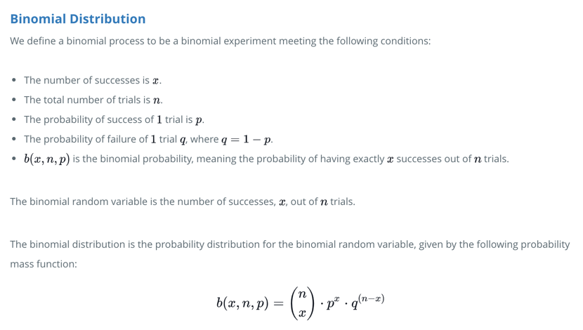
A binomial experiment (or Bernoulli trial) is a statistical experiment that has the following properties:

• The experiment consists of n repeated trials.
• The trials are independent.
• The outcome of each trial is either success (s) or failure (f).

• Expected value: np
• Variance: np(1-p)

6.3. Negative Binomial Distribution

• Negative Binomial Experiment

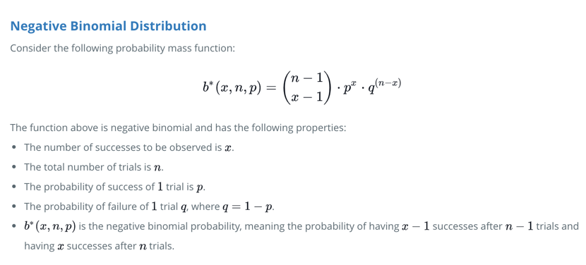
A negative binomial experiment is a statistical experiment that has the following properties:

• • The experiment consists of n repeated trials.
  • The trials are independent.
  • The outcome of each trial is either success (s) or failure (f).
  • p(s) is the same for every trial.
  • The experiment continues until x successes are observed.
    
    

If X is the number of experiments until the x^th success occurs, then X  is a discrete random variable called a negative binomial.

• Expected Value: x(1-p)/p
• Variance: x(1-p)/p^2

6.4. Geometric Distribution

The geometric distribution is a special case of the negative binomial distribution that deals with the number of Bernoulli trials required to get a success (i.e., counting the number of failures before the first success).

The geometric distribution is a negative binomial distribution where the number of successes is 1. We express this with the following formula:

g(n, p) = (1-p)^(n-1)p

• Expected Value: (1-p)/p
• Variance: (1-p)/p^2

6.5. Poisson Distribution

• Poisson Experiment

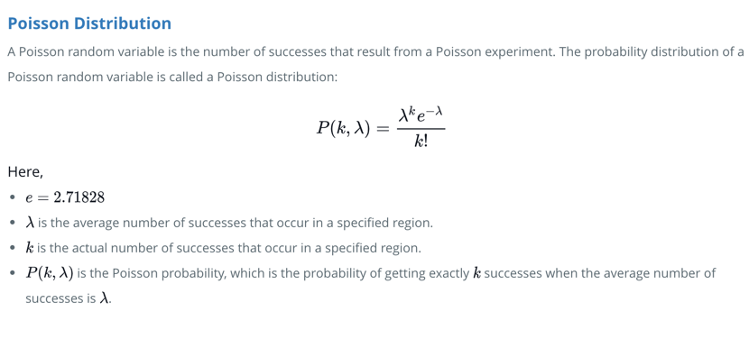
A Poisson experiment is a statistical experiment that has the following properties:

• The outcome of each trial is either success or failure.
• The average number of successes λ that occurs in a specified region is known.
• The probability that a success will occur is proportional to the size of the region.
• The probability that a success will occur in an extremely small region is virtually zero.

• Expected Value: λ
• Variance: λ

7. Conditional Probabilities

7.1. Bayes' Theorem

• p(A|B)*p(B) = p(A&B) = p(B|A)*p(A)
• p(A) = p(A&B) + p(A&^B)
  
• 1 = p(A|B) + p(^A|B)

7.2. Naïve Bayes

What does the term 'Naive' in 'Naive Bayes' mean ?

The term 'Naive' in Naive Bayes comes from the fact that the algorithm considers the features that it is using to make the predictions to be independent of each other, which may not always be the case.

• Naïve assumption:
  • P(A & B) = P(A)*P(B), A and B are independent
• 已知：
  • P(A | x1, x2,…, xi) is the proportion of P(x1, x2, …, xi | A) * P(A) = P(x1 | A)*P(x2 | A)*…*P(xi | A) * P(A)
  • P(B | x1, x2,…, xi) is the proportion of P(x1, x2, …, xi | B) * P(B) = P(x1 | B)*P(x2 | B)*…*P(xi | B) * P(B)
• 未知：
  • P(x1, x2, xi)
• 求 P(A | x1, x2,…, xi)？ P(B | x1, x2,…, xi)？Normalize proportions
  • P(A | x1, x2,…, xi) = P(x1 | A)*P(x2 | A)*…*P(xi | A) * P(A) / (P(x1 | A)*P(x2 | A)*…*P(xi | A) * P(A) + P(x1 | B)*P(x2 | B)*…*P(xi | B) * P(B))
  • P(B | x1, x2,…, xi) = P(x1 | B)*P(x2 | B)*…*P(xi | B) * P(B) / (P(x1 | A)*P(x2 | A)*…*P(xi | A) * P(A) + P(x1 | B)*P(x2 | B)*…*P(xi | B) * P(B))

8. Model Evaluation Metrics

8.1. Classification metrics

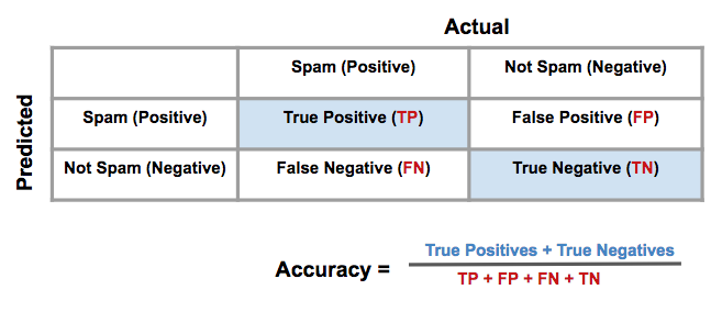
8.1.1. Confusion matrix

8.1.2. Accuracy

Measures how often the classifier makes the correct prediction. It’s the ratio of the number of correct predictions to the total number of predictions (the number of test data points).

8.1.3. Precision

Tells us what proportion of messages we classified as spam, actually were spam. It is a ratio of true positives to all positives, in other words it is the ratio of True Positives/(True Positives + False Positives)

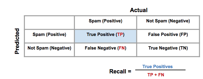
8.1.4. Recall (Sensitivity)

Tells us what proportion of messages that actually were spam were classified by us as spam. It is a ratio of true positives to all the words that were actually spam, in other words it is the ratio of True Positives/(True Positives + False Negatives)

8.1.5. Specificity

Tell us what proportion of messages that actually were not spam were correctly classified by us as not spam. It is a ratio of true negative to all the words that actually were not spam, in other words it is the ratio of True Negative/(True Negative + False Positive)

Specificity = TN/(TN+FP)

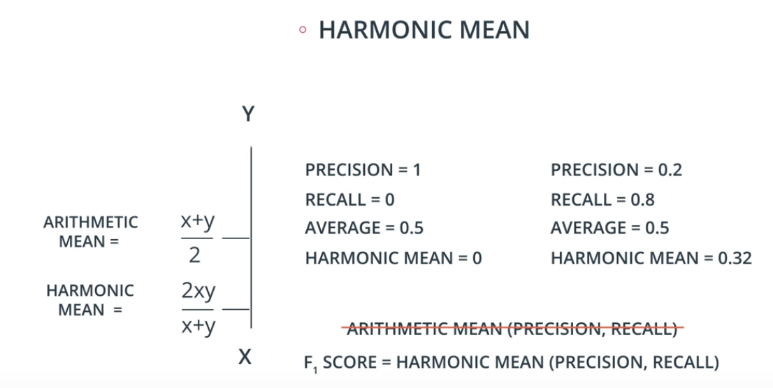
8.1.6. F1 score

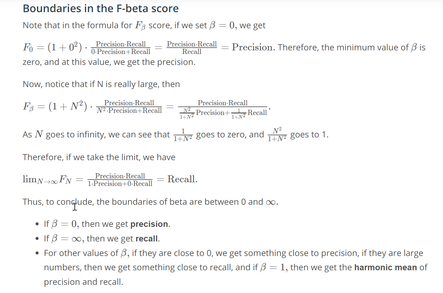
8.1.7. F_β score

• If care more about precision, you should move β closer to 0.
• If care more about recall, you should move β towards ∞.
  

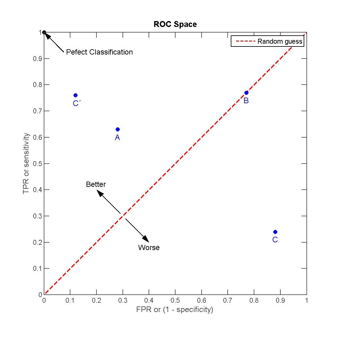
8.1.8. ROC (Receiver Operating Characteristic) curve

• True Positive rate (Recall or Sensitivity) vs False Positive rate (1 - Specificity)

8.2. Regression metrics

8.2.1. Mean Absolute Error (MAE)

8.2.2. Mean Square Error (MSE)

8.2.3. Root Mean Square Error (RMSE)

8.2.4. R² score

r² = 1 - (SE_line/SE_y) -- what % of total variation is described by the variation in x. it measures how much prediction error is eliminated when we use least-squares regression.

8.3. Cross Validation

9. Controlled Randomized Experiments

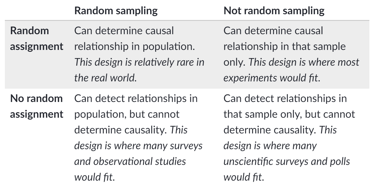
• Randomization reduce the bias by equalizing other factors that have not be explicitly accounted for in the experimental design
• Objects or individuals are randomly assigned (by chance) to an experimental group

9.1. Random Sampling Methods

• Simple random sampling
• Stratified sampling
• Clustered sampling
• Systematic random sampling

9.2. Randomized Experimental Assignment

• Completely randomized design
• Randomized block design
  • In a block design, experimental subjects are first divided into homogeneous blocks before they are randomly assigned to a treatment group. Then, within each age level, individuals would be assigned to treatment groups using a completely randomized design.
• Matched pairs design
  
  

Response bias occurs when people systematically give wrong answers.

Experimentation design: http://www.stat.yale.edu/Courses/1997-98/101/expdes.htm

9.3. Necessary Ingredients for Running Controlled Experiments

1. There are experimental units that can be assigned to different variants (test groups) with no interference;
2. There are enough experimental units;
3. Key metrics, ideally an OEC (Overall Evaluation Criterion), are agreed upon and can by practically evaluated;
4. Changes are easy to make.